Common tasks using the ImageProcessing step
This section covers some common tasks that you can accomplish using the ImageProcessing step. Topics include preprocessing to prepare the image for analysis, combining images, and creating mask images. Most of these techniques require non-default settings for the sources, destinations, regions, and output image depth or size.
 Preprocessing
You can preprocess your rough and noisy images to clean them up and help with their analysis.
Many Matrox Design Assistant analysis steps have their own preprocessing controls. In this case, you might not need to include the ImageProcessing step in your flowchart. For example, the Measurement step, the Metrology step, the ModelFinder step, and the BeadInspection step include a smoothing filter that you can adjust with a slider.
Removing spots
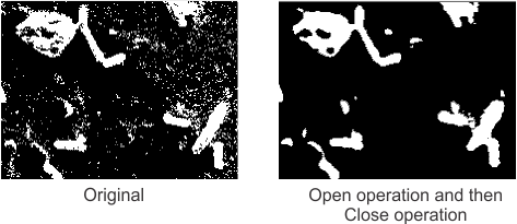
You can remove spots in your images (noise) using the ImageProcessing step's morphology operations. For example, you can use a combination of Open and Close operations with the number of iterations proportional to the size of the noise or holes to remove most of the spots in an image. The following image demonstrates this:
Removing
reflections
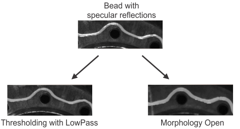
Some steps in Matrox Design Assistant (for example, the ModelFinder step) tolerate reflections in images because of their included smoothing operations. Other steps such as the BeadInspection step are more sensitive to reflections that have sharp contours; for the BeadInspection step, this is particularly the case if the contours cover a significant portion of the bead. To remove reflections, you can use a LowPass operation with a High value that is only a bit greater than the Threshold value. You could also use an Open operation where the number of iterations of the operation is modified until the glare has been removed. The follow image demonstrates what results you should expect when using these methods:
Removing the
background
Removing clutter
Sharpening
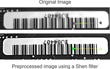
You can remove blur in your images using the filtering operations Shen and Deriche with the IIR operation input set to Sharpen. For filtering, these IIR filters are often more effective than the classic sharpen filtering operations because of newer high resolution image sensors. The following image demonstrates how you can use filters to sharpen an image:
Improving
contrast
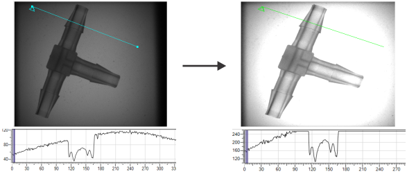
You can increase the contrast in your images to highlight distinct areas, which can help the operator see additional details and can help improve the strength of edges when using the Measurement step. You can use the LutMap WindowLeveling operation to stretch or compress a specified range of source image pixel values to fit within a newly defined range. WindowLeveling is effective if you need to draw out detail in dark areas of an image that you do not want to binarize. The following image demonstrates how WindowLeveling can increase the contrast of a translucent object to get a better view of its inner components:
Segmentation
Segmentation usually refers to clearly separating the object or feature that is to be analyzed (foreground) from the rest (background). In many cases, you can use a simple thresholding operation. A WindowLeveling operation can also be used to segment distinct areas of objects in your image. Window levelling can compress a range of input values into a smaller range of output values, removing some detail in part of the image as a result.
In the following image, you can observe from the line profile graph that the image has 3 levels of intensity. After using a WindowLeveling operation with a specified range, the segmented area's intensity will be distinct in the image.
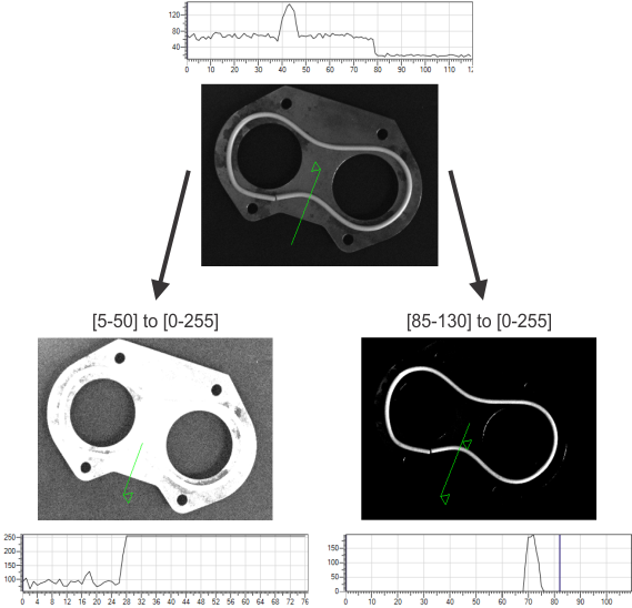
Note that it is possible to perform a similar segmentation using Threshold operations if the different levels of intensity do not overlap.
Making a mask
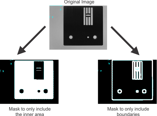
You can ignore portions of images that do not require analysis by selecting the regions on which to perform operations. Alternatively, you can create a mask derived from an object's shape. For example, you can ignore zones around edges using a combination of Threshold and Morphology operations.
To create a mask that will only include the inner area of an object, you can use a Dilate operation followed by the Logic Not operation. You can then use a Threshold operation to binarize your mask.
You can create a mask that will only include the boundaries of an object. One method is to include 2 ImageProcessing steps in your flowchart so you can modify the object in 2 different ways. In the first step, you can use the Dilate operation with a specified number of iterations on the source image to thicken the edges of the object. In the second step, you can use the Erode operation with an equivalent number of iterations to shave off pixels around the object. You can then Subtract the eroded image from the dilated one to obtain an image containing a contour of the edges of the original image. Another method to create such a mask would be to Threshold your image, detect its edges using the LaplacianEdge operation and then Dilate these edges. The advantage of this latter method is that these operations can all be performed using a single ImageProcessing step in your flowchart.
The following images shows examples of masks created using morphology and threshold operations:
To apply your mask to the original images, you can use an Arithmetic operation such as Maximum.
Superimposing
The following present 2 visualization techniques where you superimpose a pair of images.
TwoBands
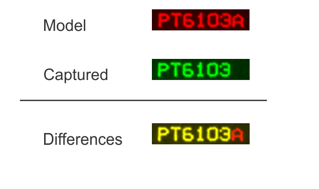
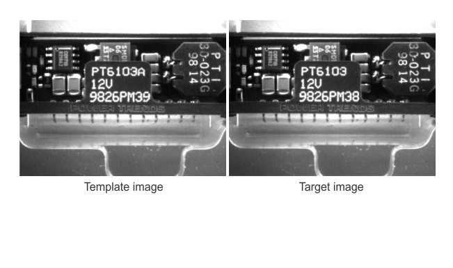
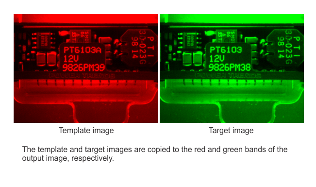
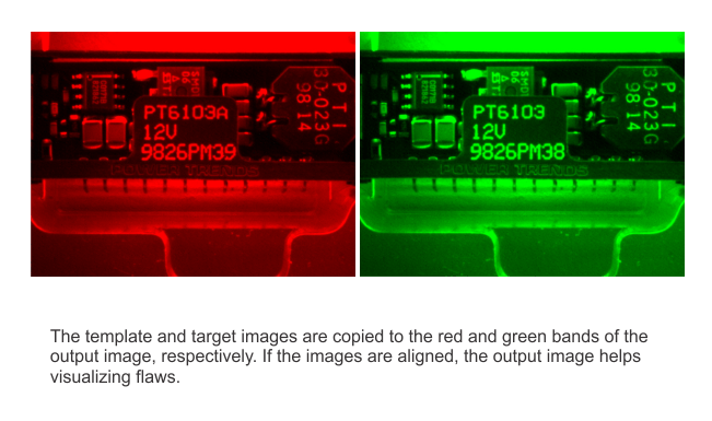
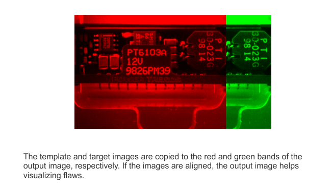
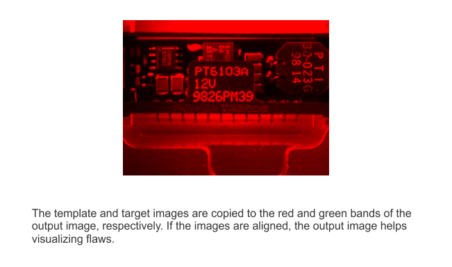
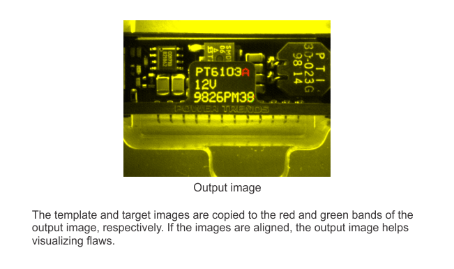
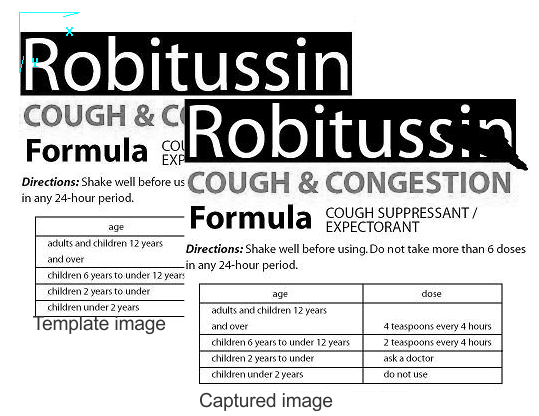
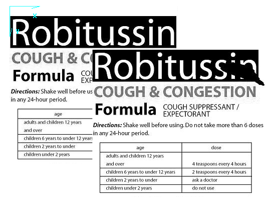
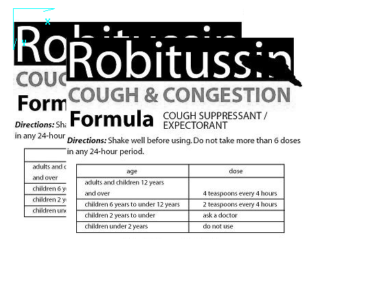
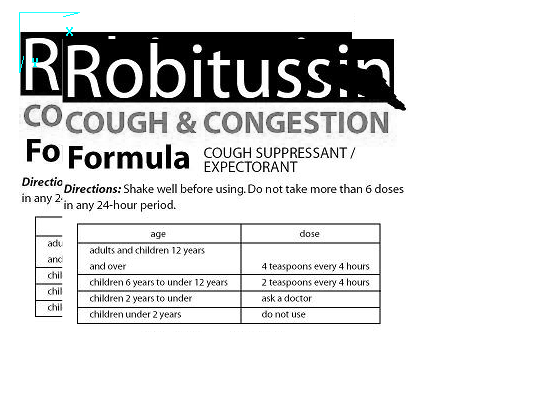
You can visually compare captured images to a template image by superimposing them. The TwoBands technique involves copying 2 aligned grayscale images into different bands of a 3-band output image. For example, if the template image is stored in the red band and the captured image is stored in the green band, then matching areas will become yellow in the output image. The features from the template image that are missing in the captured image will be red and the features in the captured image that should not be present will be green. You can also use this technique on images that have not been explicitly aligned to see if they are misaligned. The following animation demonstrates the TwoBands technique on 2 aligned grayscale images:
AlphaBlend
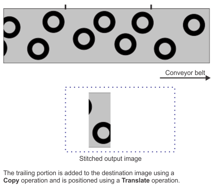
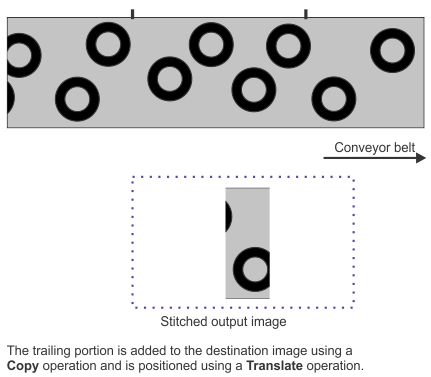
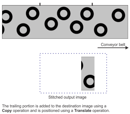
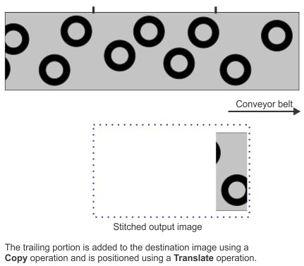
Stitching
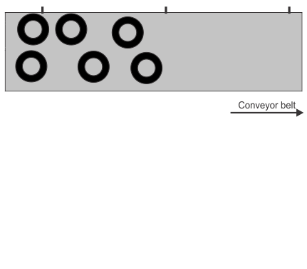
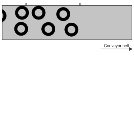
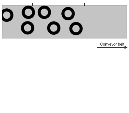
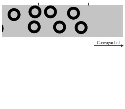
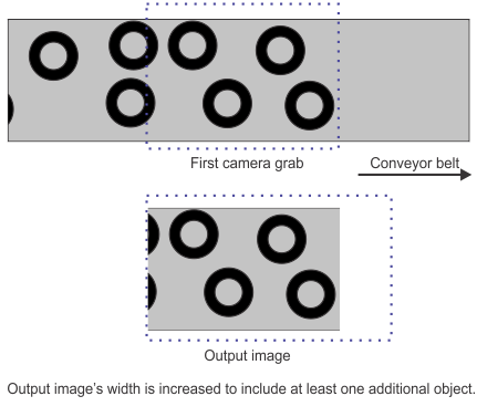
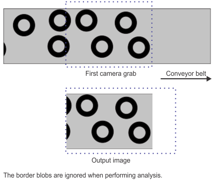
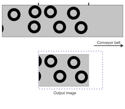
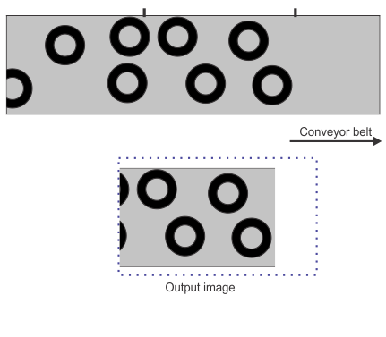
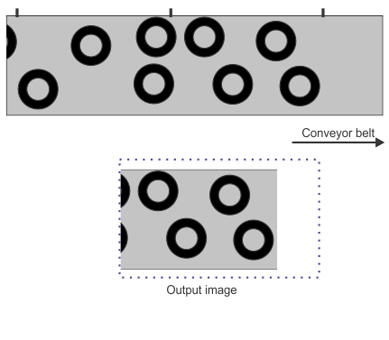
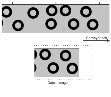
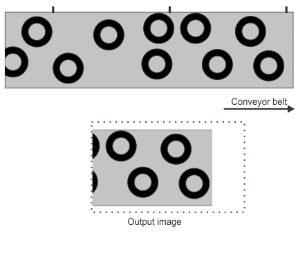
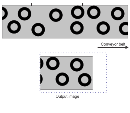
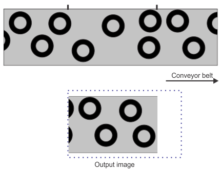
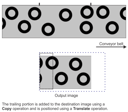
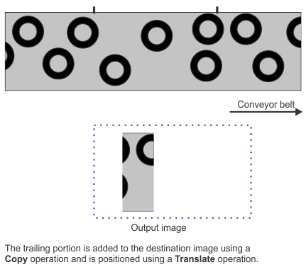
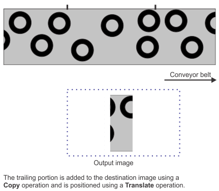
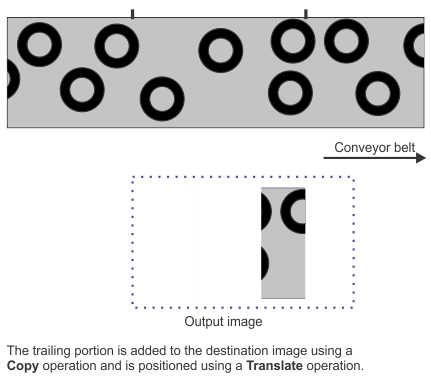
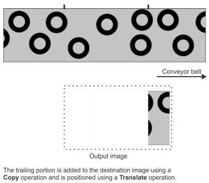
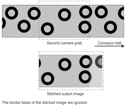
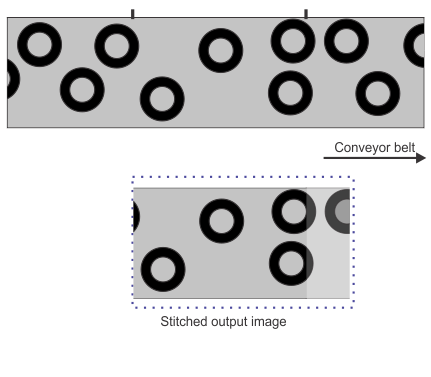
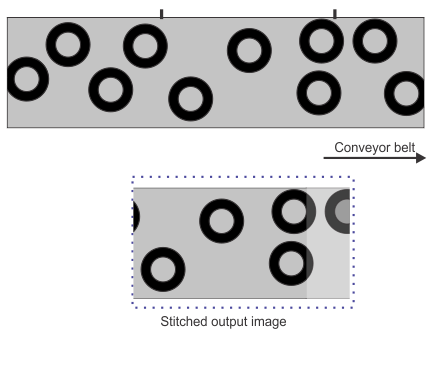
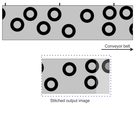
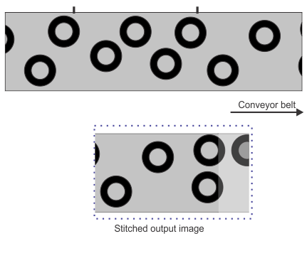
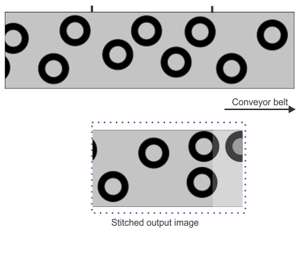
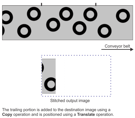
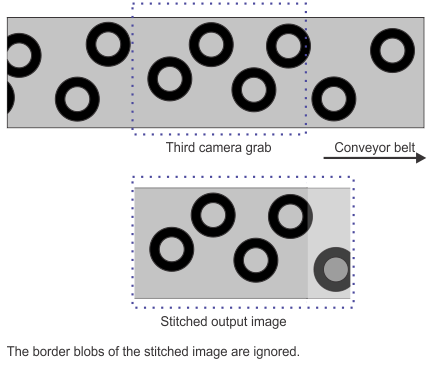
Stitching is often necessary when doing successive line scan grabs or when using a setup involving multiple cameras. You might also need to stitch your images if the objects are larger than the camera's field of view, or if your images contain partial objects at the leading and trailing edges of your images.
To stitch images with partial objects, you must first add an ImageProcessing step to your flowchart and crop the trailing portion of your grabbed image by reducing the Width of the output image; the width of this image should be equivalent to the width of a complete object. You must then store this image in a variable so you can access it in the next iteration of your flowchart's loop. In a second ImageProcessing step, and after grabbing the next image, set the step's source as None and the Width of the output image to be a sum of the width of the grabbed image and the width of the cropped image. You can then Copy the cropped image and Translate it by an amount equivalent to the width of a grabbed image. Finally, you can Copy the grabbed image to complete the stitching. The incomplete object in the current image will then be aligned with its missing portion. Note that you should use the BlobAnalysis step's Remove border blobs input before performing any analysis on your stitched images (the discarded partial blobs will be part of the previous or following stitched image). The following animation demonstrates this:


Accumulating for a temporal
filter
Color conversion
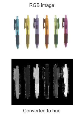
You can use the Convert operation to change the color space of images. For example, you can do this to examine the difference in hue between objects in an RGB image. If you only need to perform a few conversions, you can use the Alternate menu available in every step that has an Image input to perform a quick Hue or Luminance conversion. However, if you intend on using a converted image over multiple steps, a single usage of the Convert operation can increase the efficiency of your flowchart. The following image demonstrates how you can use the Convert operation to examine the hue of an RGB image:
Color projection
Color distance
Band difference
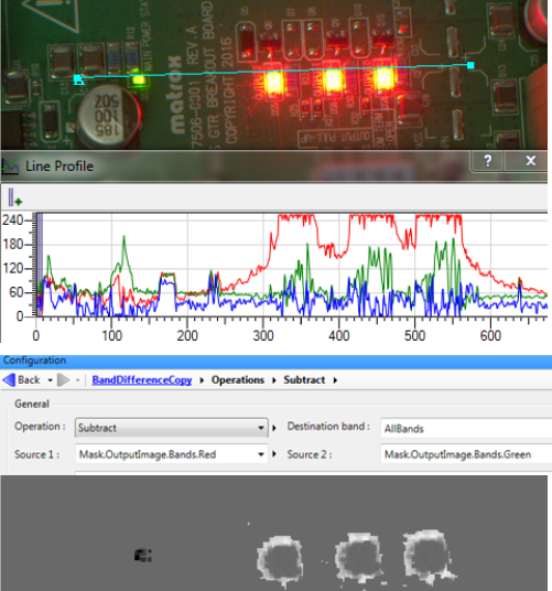
In an image where a region might be one of 2 different colors, you can quickly distinguish between them using the ImageProcessing step's Subtract operation followed by an IntensityChecker step. More specifically, calculate the difference between 2 different bands from the same color image and store the result in a 1-band signed output image. Choose 2 bands that will yield a positive result when the region is one color, and a negative result when the region is the other color. You can use the line profile tool to determine the RGB values of the colors in the image.
In the following image, the Status LED can be either orange or green. To distinguish the difference between each color we can subtract the Red band from the Green band and store this in a signed buffer. The image is transformed to black and white, which can be visualized more clearly by using the autoscale option. The black and white can then easily be distinguished by an intensity checker.
Geometry and
shape changing
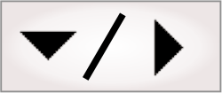
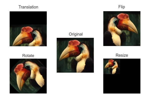
Geometric operations can properly orient, flip, translate, or resize an image. You can perform a rotation on an image and then move it so it is aligned with a template using the Rotate and Translate operations. You can perform a vertical or horizontal reflection of an image using the Flip operation to obtain its mirror image. You can create a thumbnail of an image with the Resize operation, which will change the image's scale. Resizing can also optimize your flowchart since your analysis steps will be applied to fewer pixels. Note that when resizing or rotating, you might need to change the Width and Height of the output image to accommodate the modified image. The following image shows some of the geometric modifications that you can perform:
You can also unwrap circular sections of an image to obtain a straightened and rectangular output image using the RectangularToPolar operation. For example, this is necessary when performing character recognition on images with text that is wrapped around a circle. See the PolarTransform subsection of the ImageProcessing step operations section later in this chapter subsection for more information.
Aligning
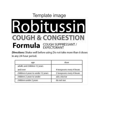
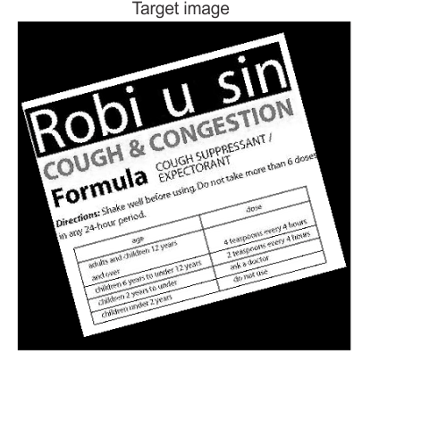
You might need to align your captured images with a template image to detect flaws in captured images. In a simple case, the angle of the template image and the captured are the same, and you can align the image with a Translate operation. In a more complex case, the angle of the template image and the capture image are not the same, and the angle needs to be corrected using the ImageCorrection step.
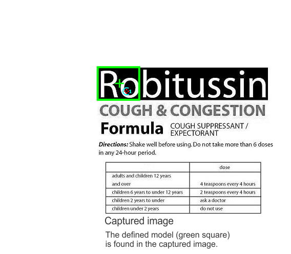
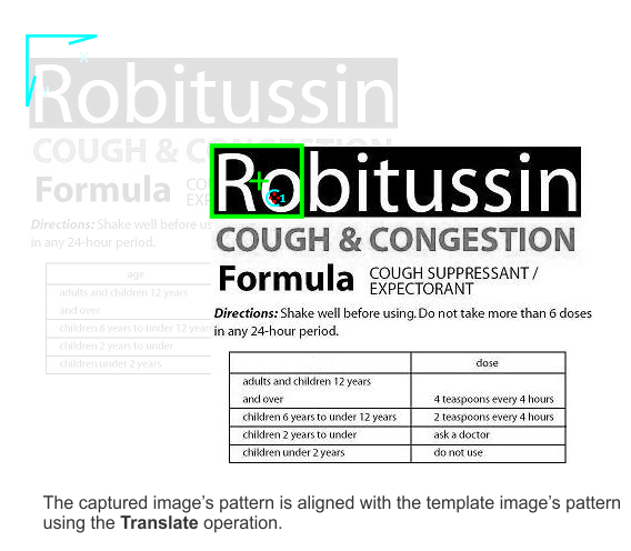
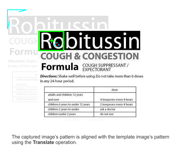
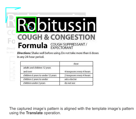
Simple aligning
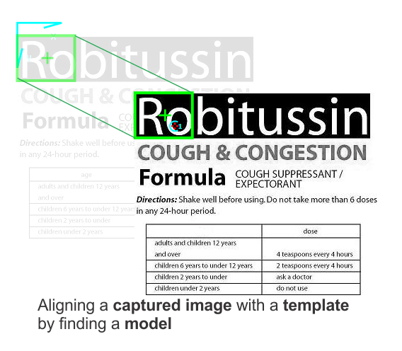
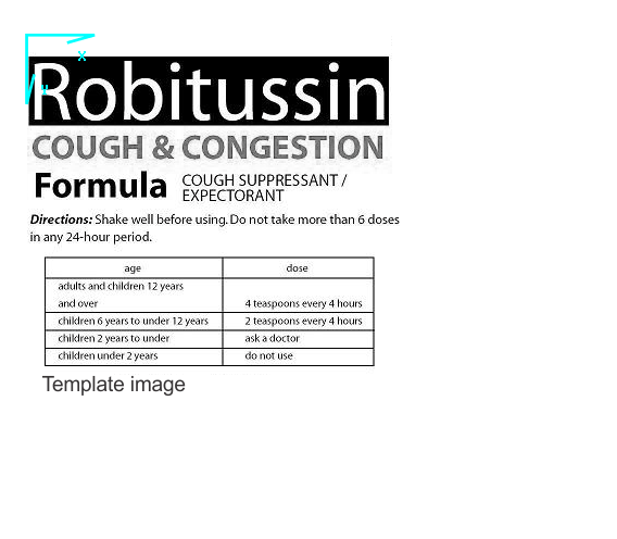
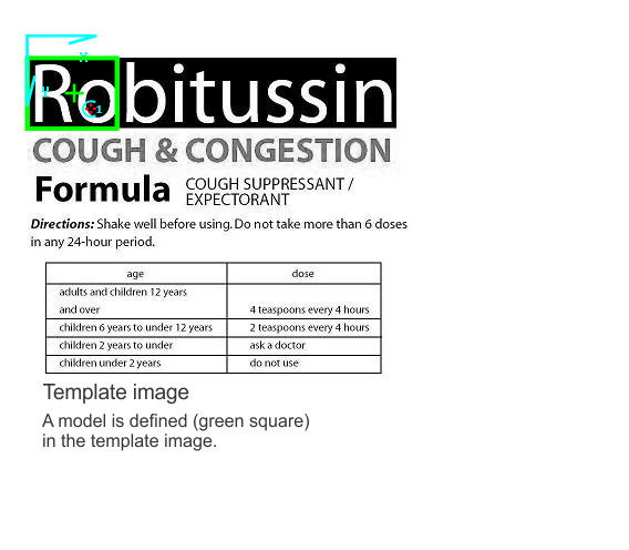
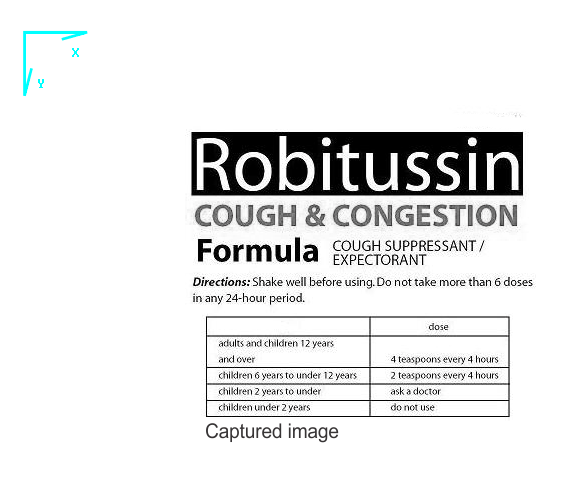
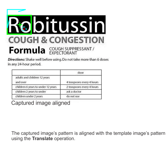
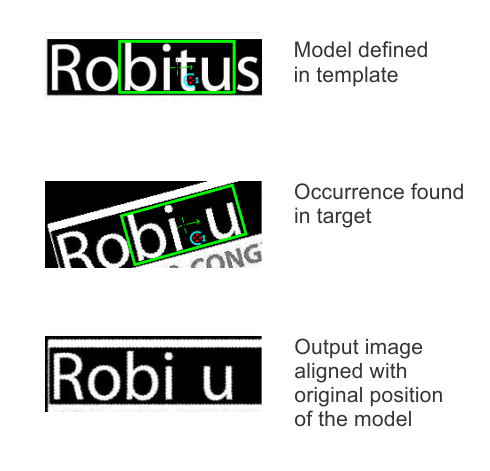
In a simple case, no rotation needs to be performed on the captured image. You can use the PatternMatching step to define a pattern in the template image. After finding a match in the captured image, you can use the Translate operation to align the match in the captured image with the original location of the model in the template image. The displacement is the difference between the coordinates of the model in the template image and the coordinates of the match in the captured image. The following animation demonstrates the simple aligning case:
Complex aligning
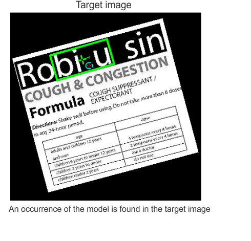
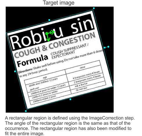
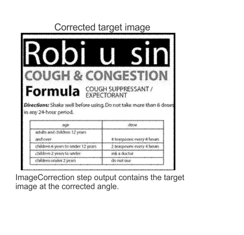
When an object in the target image appears with a rotation, you can align this object to the orientation of the same object in the template image by using an ImageCorrection step. This step transforms an image so that the target and template fixtures are aligned. Typically the ModelFinder step is used to provide the fixture in the target image, however this is not always the case. The following animation demonstrates an example with the ImageCorrection step:

Calculating
differences
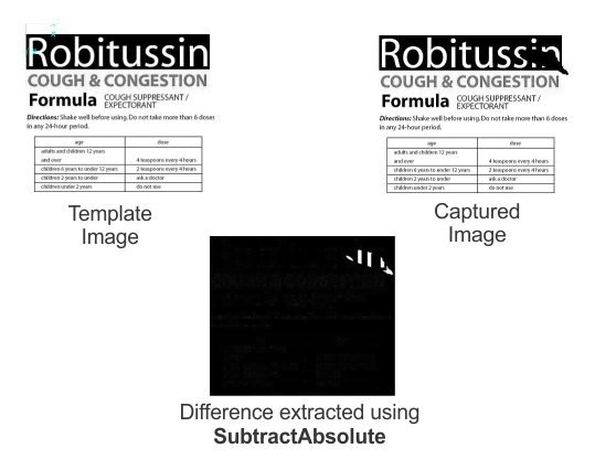
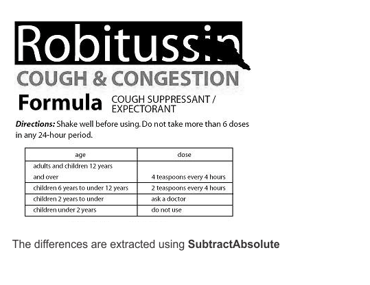
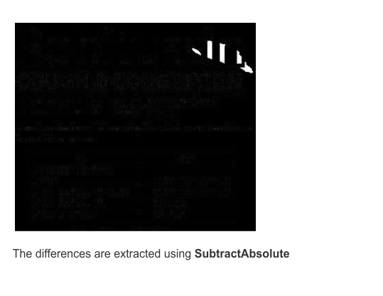
You can use the SubtractAbsolute operation with a template image and a captured image to generate an image of the differences between the 2 images. You would generally perform this after having aligned these images. The following animation demonstrates this:
Another method is to use the Subtract operation with a template image and a captured image, and set the Type of the output image to Signed16Bit. The resulting output image will either contain the captured image's missing information or the captured image's extra information. The version you get depends on which image you subtracted from the other. You should perform a Threshold operation on the output image to remove some noise, followed by a bit size conversion to compress the pixel range of the image into 8 bits.
On either version of the output image, you can then perform operations from the BlobAnalysis step to count or analyze the number of blobs. You might need to apply a Rank filter on the output image if your image still contains noise.
Inner and outer
offset
Typically, to obtain the contour of an object, you can use the LaplacianEdge or DericheEdge filter operations to detect the edges. However, if you want your contour to have a certain offset distance from the actual edge of your object, you will need another approach.
The simplest way to have an offset distance from the edge of your object is to use the Morphology Erode or Dilate operations to shrink or grow the object before using an edge filter. This can give satisfactory results for small offsets of a few pixels, but for very large offsets, the contour will be greatly distorted due to many iterations of a square morphology.
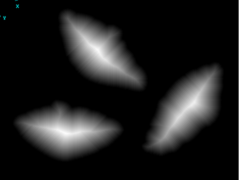
To minimize distortion in the contour, you can perform the Distance operation when using the Chamfer_3_4 distance mode. The source for the distance operation should be a binarized image (the background must have a zero value) and the object in the image cannot touch the boundaries of the image.
Note, the distance operation on an image with small objects, will generate an output image that appears almost entirely black. This is normal. To more clearly visualize the results, you can right-click on the display of the output image, and select the Autoscale option from the presented context menu. The use of Autoscale can be seen in the image below.
You will need to change the type of the output image of the Distance operation, depending on the size and shape of the object. If the resulting image shows a sharp white or black wrap around, you probably need a deeper buffer. The minimum Feret diameter of the object will determine the largest output pixel value. When using Chamfer_3_4 mode, the output value of each pixel is 3 times the distance of the pixel from the outer contour. The default Unsigned8Bit buffer is sufficient if the object has a minimum Feret diameter less than 170 pixels (2*256/3). If the object is bigger, you need to set the type of the output image to Unsigned16Bit. For more information on working with 16 bit buffers, see the Displaying images with more than 8-bits section in the Display view reference chapter .
After performing the Distance operation, you can use a TwoLevels threshold operation to extract a thin contour at a specific number of pixels from the edge. Set the operation's Threshold Low input to the number of pixels by which to offset the edge (times 3 if using Chamfer_3_4). Set Threshold High a couple of values higher than ThresholdLow. Low value, Middle value, and High value should be set to 0, 255, and 0, respectively.
To generate a contour beyond the edges of the object, invert the original binarized image using the Logic Not operation. You will then be working with the distance in the background, rather than the inside of the object.