ColorMatcher step advanced concepts
This section presents advanced information regarding concepts and settings in the ColorMatcher step.
 Color spaces
A color space is a mathematical model that typically has 3 components (bands) with which to describe color data.
Matrox Design Assistant interprets all input color data (for example, color-samples) as RGB and, by default, performs the match in RGB. However, the step can internally convert the RGB data to HSL or CIELAB (LAB) and perform the match in these color spaces (if supported by the distance type). Use the Configuration pane to modify the color space in which to perform the match.
Note that you can use the ImageProcessing step for simple conversions between RGB and HSL, however, the ColorMatcher step expects an RGB input image.
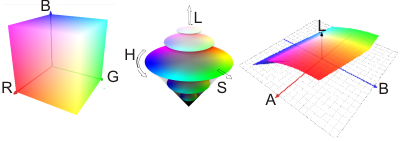
RGB
RGB is based on red, green, and blue color component (band) values. Typically, these components are directly used for acquiring and displaying color. For example, when displaying a color image, the first band is routed to the monitor's first output channel (usually red), the second band to the second channel (usually green), and the third band to the third channel (usually blue).
The RGB color space can be seen as a cube with a red, green, and blue axis. Colors located at the origin, [0, 0, 0], are considered to be black, while colors located at [255, 255, 255] (for an 8-bit buffer) are considered to be white. All other colors can be represented as a combination of red, green, and blue values within this range.
Acquisition and display devices can render RGB data differently. Since RGB maps to such devices, it is a device-dependent color space.
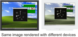
Theoretically, there are as many RGB color spaces as there are color devices. Although there will always be some variance, color devices typically adhere to certain internationally accepted standards. To interpret color space data, Matrox Design Assistant uses standard RGB specifications (sRGB), as defined by the International Electrotechnical Commission (IEC) Project Team 61966-2-1.
HSL
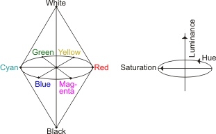
HSL is established from an RGB color model, but is based on hue, saturation, and luminance color component (band) values. Since such components are generally more intuitive, HSL can be seen as a color space designed to mimic the human way of describing colors. Like RGB, HSL is device-dependent.
In RGB, every color is a mixture of red, green, and blue, which can make it difficult to ascertain the exact component values of a particular color. However, in HSL, the color's hue is stored as a separate component (H), which is represented as an angular position on a circular color disk. The other components control only the color's purity (S) and brightness (L), which can be used to alter the color's quality, but not the color's basic hue. This type of band independence can make color manipulation much simpler with HSL. Most color pickers that allow for an interactive manipulation of colors represent the color with HSL.
Note that matching colors with the hue (color) band only can sometimes solve certain problems, such as helping to distinguish matches between dark orange and bright orange, which can, for example, be difficult in RGB. Also, matching the hue independently of the luminance can be useful if your image has non-uniform lighting, shadows, or highlights. For more information, see Bands input.
CIELAB
CIELAB (also known as LAB) is based on the color's luminance (L), its position between red and green (A), and its position between yellow and blue (B). Unlike RGB and HSL, CIELAB is intended to be device-independent, and was developed as a distinct color model intended to represent a completely human interpretation of color by using statistical data taken from visual experiments. Color differences in CIELAB vary proportionally with human perception. For example, if 2 colors are at a distance of 5, they will appear roughly 5 times as different as 2 colors at a distance of 1. CIELAB was designed to be perceptually uniform, making it a good space to measure color difference.
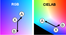
Since CIELAB is based on color perception, its mathematical model better represents how humans distinguish color, and color differences are more meaningful. This can be seen in the following example, where you have to choose which color, A or B, is closer to color X.
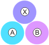
Mathematically, color A is the closest color, in an RGB color space. However, color B is intuitively closer, which is also what the distance in the CIELAB color space mathematically represents.
It can be preferable to use CIELAB over RGB since, like HSL, you can use CIELAB to discard the luminance (band L), and perform color matching with only band A and band B. For more information, see Bands input. Also, CIELAB can be more robust with colors that are visually alike, especially for minor color differences. For example, when matching a red target among color-samples with similar shades of red, CIELAB can outperform RGB and HSL.
With CIELAB, distances have been standardized by the International Commission on Illumination (CIE). A color distance of 1 with CIELAB corresponds to the smallest possible color difference a human can perceive.
Bands input
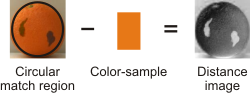
Color distance
Color distance refers to the numerical difference between the
color of the match region and the color of the color-sample. After
running the ColorMatcher step, you can
get this numerical difference with the distance result. You can
also visualize the difference by viewing the distance image, which
you can select by clicking on the
Change display image (![]() ) toolbar button in the
Project toolbar. The distance image displays the difference
in color as a grayscale value; the more different the colors, the
brighter the distance image will be. This can, for example, allow
you to quickly spot potential flaws.
) toolbar button in the
Project toolbar. The distance image displays the difference
in color as a grayscale value; the more different the colors, the
brighter the distance image will be. This can, for example, allow
you to quickly spot potential flaws.
Since the ColorMatcher step uses the color distance to match colors, modifying the type of color distance calculation can be a useful way to adjust the match operation to suit your application. Although the default distance calculation is typically sufficient, you can choose one of several different types of distance calculations: Euclidean, Manhattan, Mahalanobis, or DeltaE. You can also choose an advanced distance type (CMC... or CIE...), as established by the standards of the International Commission on Illumination (CIE). To change the distance type, use the Configuration pane.
If necessary, you can normalize distance results. For more information, see the Distance normalization subsection of this section.
Note that if your application only requires the distance between simple colors, you can use the ImageProcessing step.
Euclidean
distance
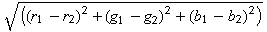
A Euclidean distance is the square root of the sum of the squared differences between the color of the match region and the color of the color-sample. A Euclidean distance is generally regarded as a well-known standard distance calculation.
The following example illustrates how the distance between a green point, indicated by a circle, and 2 other green points, indicated by a triangle and a square, is measured with a Euclidean calculation.
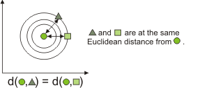
A Euclidean distance can be represented with the following formula:
Manhattan
distance
A Manhattan distance (also known as a City Block distance) is the sum of the absolute value of the differences between the color of the match region and the average color of the color-sample. A Manhattan distance is generally considered the simplest distance calculation and is typically appropriate for calculating color distances between hue (H) bands in HSL.
The following example illustrates how the distance between a green point, indicated by a circle, and 2 other green points, indicated by a triangle and a square, is measured with a Manhattan calculation.
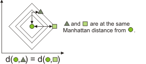
A Manhattan distance can be represented with the following formula:

In the Euclidean and Manhattan distance formula, r represents the first color component of the match region (subscript 1) and color-sample (subscript 2), g represents the second color component of the match region (subscript 1) and color-sample (subscript 2), and b represents the third color component of the match region (subscript 1) and color-sample (subscript 2).
Note that in HSL the color's hue is stored as a separate component (H) represented as an angular position on a circular color disk. Therefore the distance between colors is equal to the smallest angular difference, rather than the absolute value of the difference.
Mahalanobis
distance
A Mahalanobis distance is calculated between the color of the match region and the covariance of the color-sample. A Mahalanobis distance is generally regarded as a slower, though more robust distance calculation typically used for elongated color-samples.
The following example illustrates how the distance between a green point, indicated by a circle, and 2 other green points, indicated by a triangle and a square, is measured with a Mahalanobis calculation.
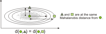
A Mahalanobis distance can be represented with the following formula:
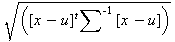
Here, x represents the match region, u represents the average of the color-sample, and sigma is for the covariance matrix of the color-sample color.
The distance calculated for Mahalanobis, between a color and a distribution of colors (covariance), is similar to a Euclidean distance between the mean of the 2 colors, but weighted by the inverse of the covariance of the distribution. This implies that the more a color distribution varies in a direction within the color space, the less significant the distance is in that direction.
Since the covariance matrix of the color-sample is used, the color-sample should typically be a distribution of colors, such as an image, and not a single solid color (a custom color). However, if you provide a custom color as the color-sample, Mahalanobis behaves very much like Euclidean and will yield similar results.
Delta-E distance
Advanced CIE
distance types
Choosing a
distance type
Choosing the most appropriate distance type with which to calculate color distances depends on many factors, including the color space of your data, the background, and the particularities of your application. Typically, you should use a Euclidean distance for RGB and CIELAB color spaces, and a Manhattan distance for HSL. You should use a Mahalanobis color distance when dealing with closely-related colors, and that are not expressed in HSL.
The following example illustrates a match operation that uses an RGB image of a grapefruit. As indicated, for RGB colors a Euclidean distance is typically sufficient; however, in this specific case, a Mahalanobis distance is preferable.
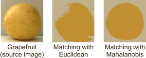
In the source image, the color of the background and some parts of the grapefruit are similar; this makes Mahalanobis yield better results, since the covariance of the image is used. The pixels of the grapefruit correspond roughly to a distribution of shades of yellow, therefore, with a Mahalanobis distance, shades of yellow are considered to be closer to the grapefruit than other colors. To illustrate this point, the following image shows 2 groups of pixels displayed in RGB; one group is from the image's background, and the other is from the grapefruit.
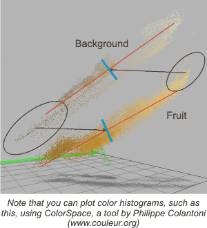
For each group of pixels (background and grapefruit), this image shows:
-
The first principal component (the red line), which represents the direction of greatest standard deviation.
-
The mean color, indicated by the intersection of the blue line with the principal component.
Encircled in black, on the left, are the background pixels that will match the grapefruit, being closer by Euclidean distance to the grapefruit's mean color. Encircled in black, on the right, are the grapefruit's pixels that will match the background, being closer by Euclidean distance to the background's mean color. However, with a Mahalanobis distance, any distance oriented parallel to the principal component (the red lines) will be scaled by the inverse of the standard deviation. Therefore the encircled pixels will match with the correct group (background or grapefruit), yielding a better matching result.
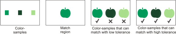
Color tolerance
The color tolerance refers to the maximum color distance, between the color-sample and the match region, allowed for a successful match. The greater the color tolerance, the greater the distance (difference) between matching colors can be. For example, if your match region is green, you can set the distance tolerance to 0 to only match with the exact same green. However by increasing the tolerance, you can match with colors that are progressively different than the original.
To specify the match's color tolerance, you must set the Tolerance mode property, which indicates how to interpret the tolerance value, which you must set with the Tolerance property. When setting the tolerance value, you must consider the specified distance type and color space. For example, a distance tolerance of 1 when using a Mahalanobis distance type is not the same as when using a Manhattan distance type.
If you set Tolerance mode to Absolute, the match uses the Tolerance value exactly as specified.
If you set Tolerance mode to Relative, the smallest distance between a sample and its neighbouring color-samples is multiplied by 0.5; this value is then multiplied by the Tolerance value and the result is the color tolerance used by the match. For Relative, if you set the Tolerance to Auto, the color tolerance value used by the match is 1.
If you set the Tolerance mode to SampleStdDev, the standard deviation of the colors within the color-sample is multiplied by the Tolerance value and the result is the color tolerance used by the match. For SampleStdDev, if you set the Tolerance to Auto, the color tolerance used by the match is 3.
The sample list's Match Radius indicates what absolute distance can be considered a match. Comparing this value to the distance output can help tune a sample's tolerance when using tolerance modes other than Absolute since it is then hard to gauge how to change the tolerance.
Match strategy
The match strategy refers to whether the match is performed using areas, pixels, or histograms. To set the match strategy, use the Match property in the Configuration pane.
Areas
When matching using areas, color statistics are calculated (typically the mean/average) for each match region and for each color-sample, and the color distance between each match region and each color-sample is taken. The resulting distances determine the score of the color-samples. The closer the colors, the higher the score. If a distance is not within a color-sample's color tolerance, the color-sample's score is 0%. The color-sample with the highest score is the match region's best-matched color-sample. In the following example, the match region's average color is calculated, and then matched with color-sample 1, which is the closest (best-match) color.
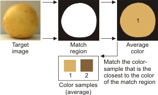
In this case, you should accurately define the match region, and it should generally consist of the required color, as indicated in the example above.
Pixels
When matching using pixels, color statistics are calculated (typically the mean/average) for each color-sample, and the color distance between each pixel in each match region and each color-sample is taken. Each target pixel then votes for the color-sample with the closest color, and which is also within the color tolerance. The number of votes that a color-sample accumulates determines its score. The greater the number of votes, the higher the score. The color-sample with the highest score is the match region's best-matched color-sample. In the following example, each target pixel votes for the color-sample that has the closest color. In general, grapefruit pixels will vote for color-sample 1, while background pixels will vote for sample 2. Since there are more grapefruit pixels, color-sample 1 is the best-match.
Since this match strategy operates on a pixel-by-pixel basis, it provides more detailed results (for each pixel) than matching using areas and is generally more robust (but slower). A pixel strategy is also less sensitive towards the accuracy of the match regions; as indicated in the example above, the target need not consist of only the grapefruit.
Histograms
When matching using histograms, color histograms are calculated for each match region and for each color-sample. A match score is then calculated between each match region histogram and the color-sample histograms. The color-sample with the highest match score is the match region's best-matched sample. When using a histogram strategy, you must set the Tolerance mode property to Absolute.
With a histogram strategy, pixel values are grouped together by subdividing their color space into bins of equal size. You must specify the number of bins for each color band using the BinsBand1, BinsBand2 and BinsBand3 inputs accessible from the Properties pane. The match score is based on the comparison of histogram frequencies for each bin, rather than each individual pixel value. A histogram strategy is generally the most robust when dealing with color-samples that contain a mixture of colors.
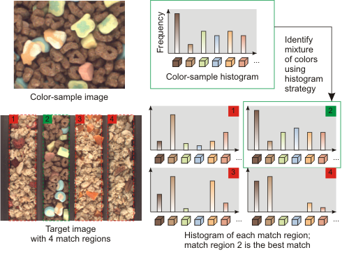
Note that the histograms shown above are approximations intended for explanatory purposes.
Distance
normalization
Color distances are calculated as numerical floating-point values. You can however normalize (remap) distance values according to a multiplicative factor, using the Distance normalization property (from the output images settings in the Configuration pane). You can specify a specific normalization value (multiplicative factor) or Maximum, which normalizes distances according to the greatest calculated distance. By default there is no normalization.
In certain cases, normalizing distances can help differentiate similar colors when viewing the distance output image, which is a grayscale image.
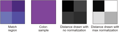
Once normalized, the resulting grayscale values drawn in the distance image do not represent a precise color distance and should never be interpreted as such. You can however make the general conclusion that the higher (brighter) the grayscale value, the greater the color distance. You can therefore consider normalization as remapping distance values to obtain an image with discernible grayscale differences that you can then use for other types of grayscale processing, such as thresholding and blob analysis.